
Overview
High-quality climate data is the foundation of reliable Species Distribution Models (SDMs). This article introduces the downscaled bioclimatic datasets produced by the Queensland Government and published in Toombs et al. (2026), and how to use them effectively in EcoCommons tools or other workflows.
These datasets provide:
- Fine spatial resolution climate data (5 km)
- Bias-corrected projections
- Ecologically meaningful variables (Bioclim 01 – Bioclim 19)
- Both dynamical and statistical downscaling, combined - a key point of difference from most global bioclim datasets
What You Get
Each dataset includes:
Climate variables
- Temperature (min, max, mean)
- Precipitation
Derived bioclim variables
- Bioclim 01 – Biolclim 19 (ecologically meaningful summaries)
Temporal coverage
- Full span: 1975–2099
- Historical baseline (used for climate-change comparisons): 1995–2014
- Historical simulation period: 1960–2014
- Future projection period: 2015–2100
Scenarios
- SSP1-2.6 (sustainability)
- SSP2-4.5 (middle-of-the-road)
- SSP3-7.0 (regional rivalry, medium-high emissions)
⚙️ How to Use in EcoCommons
In SDMs (via the platform)
- Select SDM experiment > Upload species occurrence data
- Select Climate and Environmental dataset > Find the collection and pick current
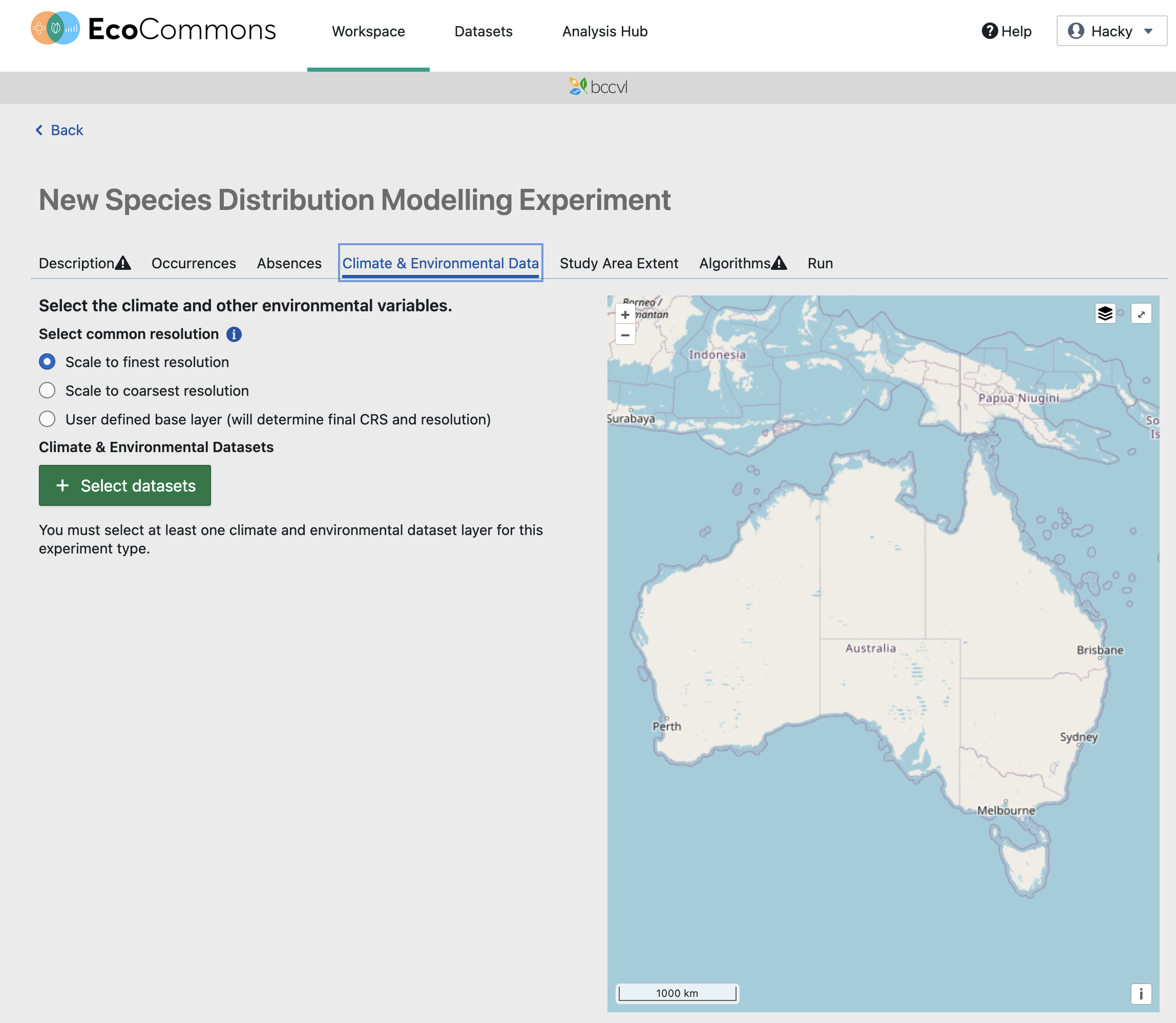
- Choose bioclim variables (Bioclim 01 – Bioclim 19) relevant to your species' ecology — you don't need all 19
- Select your study region
- Run your SDM (e.g. biomod2 with GLM or ANN) experiment
- Select CC experiment
- Select Climate and Environmental dataset > Find the collection and pick future projections
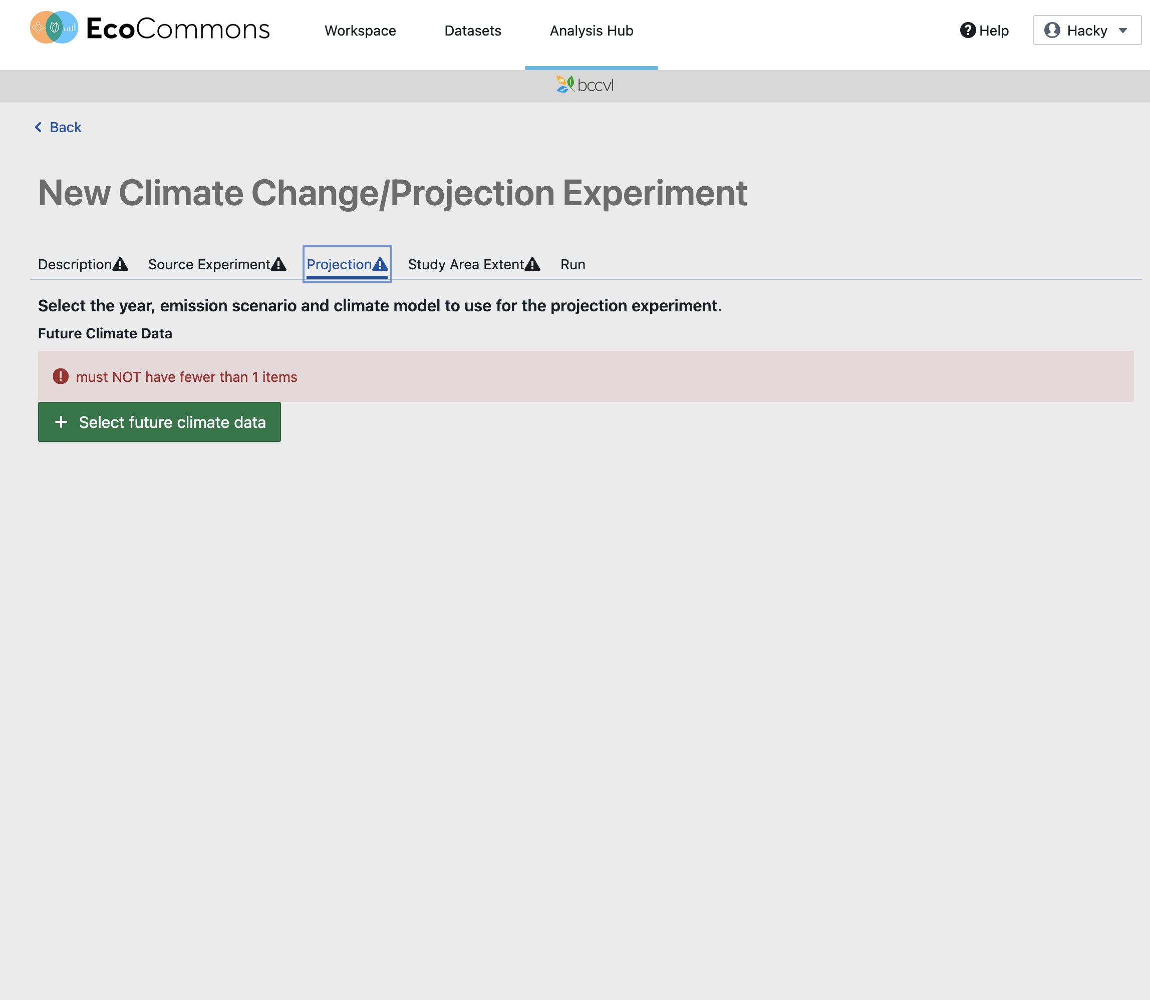
- Select GCM(s) and scenario(s) — ideally more than one model, not just the ensemble mean
- Run experiment
- Compare current vs. future outputs
In your own code environment (via URL)
The dataset and its supporting products are openly available for direct download/API access rather than only through the EcoCommons interface.
Pull these directly into R or Python (e.g. terra/raster in R, xarray/rioxarray in Python) if you want to work outside the EcoCommons GUI — useful if you're scripting a reproducible pipeline rather than using the point-and-click platform.
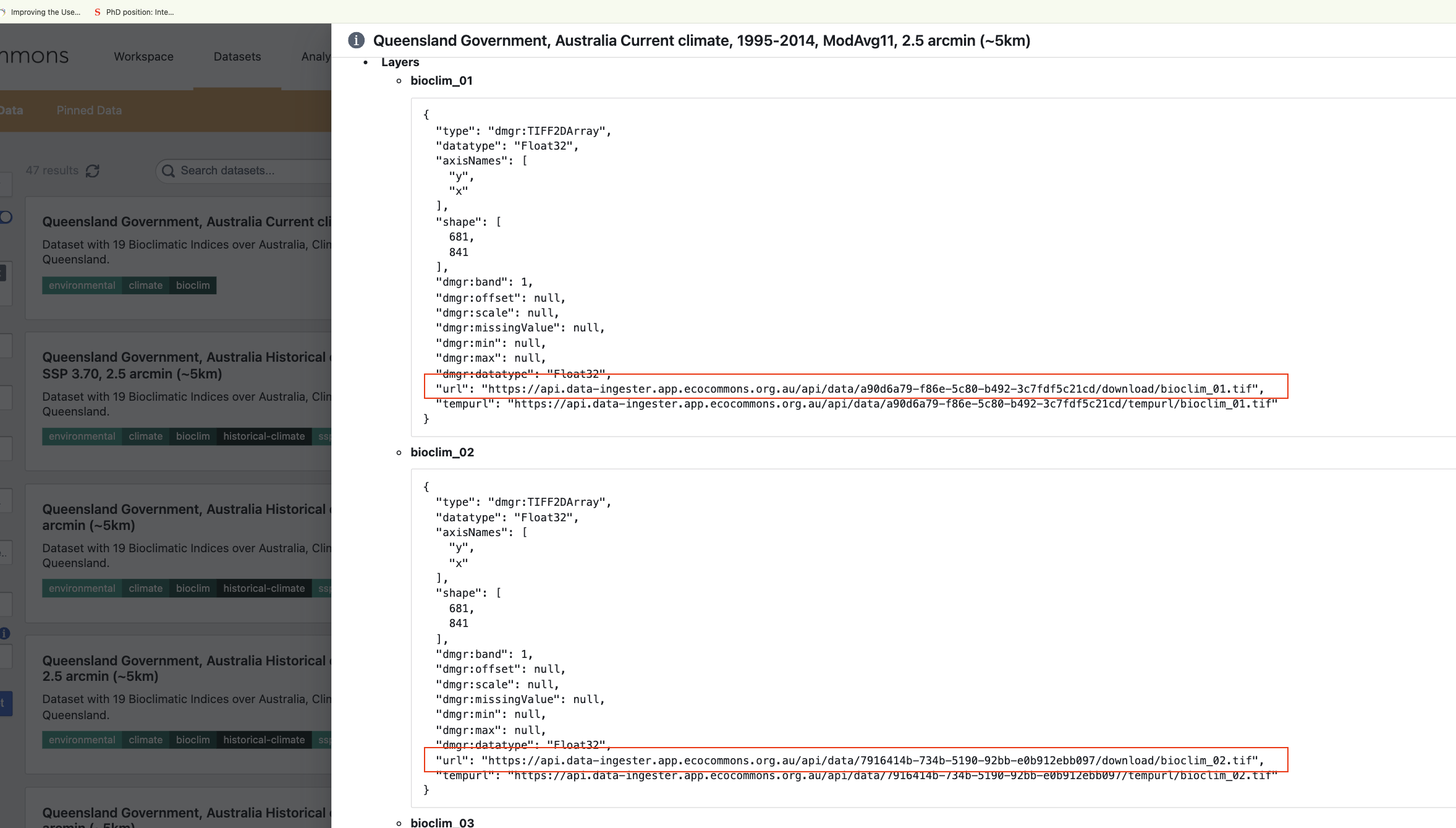
Individual bioclim layers are also served as direct-download GeoTIFFs via the EcoCommons data-ingester API, e.g. BIO1 (annual mean temperature):https://api.data-ingester.app.ecocommons.org.au/api/data/a90d6a79-f86e-5c80-b492-3c7fdf5c21cd/download/bioclim_01.tif
R (using terra)
# install.packages("terra") if not already installed
library(terra)

url <- "https://api.data-ingester.app.ecocommons.org.au/api/data/a90d6a79-f86e-5c80-b492-3c7fdf5c21cd/download/bioclim_01.tif"
dest <- "bioclim_01.tif"

download.file(url, destfile = dest, mode = "wb")
bio1 <- rast(dest)
plot(bio1, main = "BIO1 - Annual Mean Temperature")
Python (using rioxarray)
import requests
import rioxarray as rxr

url = "https://api.data-ingester.app.ecocommons.org.au/api/data/a90d6a79-f86e-5c80-b492-3c7fdf5c21cd/download/bioclim_01.tif"
dest = "bioclim_01.tif"

response = requests.get(url, stream=True)
response.raise_for_status()
with open(dest, "wb") as f:
    for chunk in response.iter_content(chunk_size=8192):
        f.write(chunk)

bio1 = rxr.open_rasterio(dest)
bio1.plot()
Swap the respective url to grab other indices. The image below shows the url option. Use combination function to loop every layer, to have one neat custom function to call all needed data layer in one go.
Using Multiple Climate Models
A key feature of this dataset is that it draws on 11 CMIP6 GCMs, dynamically downscaled to 10 km with CSIRO's CCAM, then statistically downscaled and bias-corrected to 5 km (15 model runs in total, since some GCMs were run in multiple variants or coupling modes).
Models used in this Data including their full name, resolution (in degrees), ensemble member and CCAM setup (atmosphere only or ocean-coupled).
| CMIP6 Model | Model full name | Resolution (in degrees) | Ensemble member | CCAM setup |
|---|---|---|---|---|
| ACCESS-ESM1.5 | Australian Community Climate and Earth System Simulator, version 1.5 | 1.875 × 1.25° | r6i1p1f1 r20i1p1f1 r40i1p1f1 | Atmospheric atm-ocean coupled atm-ocean coupled |
| ACCESS-CM2 | Australian Community Climate and Earth System Simulator, version 2 | 1.875 × 1.25° | r2i1p1f1 | atm-ocean coupled |
| CMCC-ESM2 | Centro Euro-Mediterraneo sui Cambiamenti Climatici | 0.9 × 1.25° | r1i1p1f1 | Atmospheric |
| CNRM-CM6-1-HR | Centre National de Recherches Météorologiques Coupled Global Climate Model, version 6.1, high-resolution | 0.5 × 0.5° | r1i1p1f2 r1i1p1f2 | Atmospheric atm-ocean coupled |
| EC-Earth3 | European Community Earth-System Model, version 3 | 0.8 × 0.8° | r1i1p1f1 | Atmospheric |
| FGOALS-g3 | Flexible Global Ocean-Atmosphere-Land System Model, grid point version 3 | 2.5 × 2.5° | r4i1p1f1 | Atmospheric |
| GFDL-ESM4 | Geophysical Fluid Dynamics Laboratory Earth System Model, version 4 | 1 × 1° | r1i1p1f1 | Atmospheric |
| GISS-E2-1-G | Goddard Institute for Space Studies Model E2.2 G | 2 × 2.5° | r2i1p1f2 | Atmospheric |
| MPI-ESM1-2-LR | Max Planck Institute Earth System Model, version 1.2, low resolution | 1.9 × 1.9° | r9i1p1f1 | Atmospheric |
| MRI-ESM2-0 | Meteorological Research Institute Earth System Model, version 2.0 | 1.125 × 1.125° | r1i1p1f1 | Atmospheric |
| NorESM2-MM | Norwegian Earth System Model, version 2, 1° resolution | 1 × 1° | r1i1p1f1 r1i1p1f1 | Atmospheric atm-ocean coupled |
(Full ensemble-member codes are in the paper's Table 1 if you need them.)
Why this matters
- Different GCMs represent different plausible futures — e.g. wetter vs. drier trajectories
- Using only the ensemble mean smooths out real inter-annual variability
- In the paper's own greater glider case study, both the driest (ACCESS-ESM1-5) and wettest (EC-Earth3) individual models predicted larger range losses than the ensemble mean did
Recommended approach
- Run your SDM across a selection of individual GCMs, not just the mean
- A practical shortcut is the "storyline" approach — pick a wet-extreme and a dry-extreme model to bracket the uncertainty
- Calculate the ensemble mean and range only at the end of your analysis, not before
Variable description
The 19 bioclimatic indices, their units, the climate variables that they are derived from and a short description of what they measure (Noce et al. 2020).
| Bioclimatic Index | Unit | Derived From | Description |
|---|---|---|---|
| Bioclim 01 - Annual Mean Temperature | °C | Min temp, Max temp | Indicates the total amount of energy inputs for the ecosystems in a year. |
| Bioclim 02 - Mean Diurnal Range (Mean of monthly (max temp − min temp)) | °C | Min temp, Max temp | Indicates the daily fluctuations of temperatures. Has a strong influence on ecosystems. |
| Bioclim 03 - Isothermality (BIO2/BIO7 × 100) | % | Min temp, Max temp | Quantifies how large the day-to-night temperatures oscillate relative to annual oscillations among extreme (warmest and coldest) months. |
| Bioclim 04 - Temperature Seasonality (Standard Deviation × 100) | °C | Min temp, Max temp | Measures the temperature change throughout the year. The larger the standard deviation value, the greater the variability of temperature within the year. |
| Bioclim 05 - Max Temperature of Warmest Month | °C | Max temp | The maximum temperature of the warmest month of the year. Note that the warmest month can be different from year to year. |
| Bioclim 06 - Min Temperature of Coldest Month | °C | Min temp | The minimum temperature of coldest month of the year. Note that the coldest month can be different from year to year. |
| Bioclim 07 - Temperature Annual Range (BIO5 - BIO6) | °C | Min temp, Max temp | Measures the range of temperature between the warmest and coldest months, i.e. the difference between BIO5 and BIO6. |
| Bioclim 08 - Mean Temperature of Wettest Quarter | °C | Min temp, Max temp, Precipitation | The mean temperature over the wettest quarter of a year (as defined by the middle month of a three-month period within a year). Note that the wettest quarter can be different from year to year. |
| Bioclim 09 - Mean Temperature of Driest Quarter | °C | Min temp, Max temp, Precipitation | The mean temperature over the driest quarter of a year (as defined by the middle month of a three-month period within a year). Note that the driest quarter can be different from year to year. |
| Bioclim 10 - Mean Temperature of Warmest Quarter | °C | Min temp, Max temp | The mean temperature over the warmest quarter of a year (as defined by the middle month of a three-month period within a year). Note that the warmest quarter can be different from year to year. |
| Bioclim 11 - Mean Temperature of Coldest Quarter | °C | Min temp, Max temp | The mean temperature over the coldest quarter of a year (as defined by the middle month of a three-month period within a year). Note that the coldest quarter can be different from year to year. |
| Bioclim 12 - Annual Precipitation | mm | Precipitation | The total amount of precipitation inputs into an ecosystem and its water cycle, expressed in mm/year. |
| Bioclim 13 - Precipitation of Wettest Month | mm | Precipitation | Month with the highest total precipitation in a year. Note that the wettest month can be different from year to year. |
| Bioclim 14 - Precipitation of Driest Month | mm | Precipitation | Month with the lowest total precipitation in a year. Note that the driest month can be different from year to year. |
| Bioclim 15 - Precipitation Seasonality (Coefficient of Variation) | % | Precipitation | The ratio of the standard deviation and the mean monthly average precipitation over the 12 months of a year. To avoid division by 0, the denominator is increased by 1. |
| Bioclim 16 - Precipitation of Wettest Quarter | mm | Precipitation | The total precipitation over the wettest quarter of a year (as defined by the middle month of a three-month period within a year). Note that the wettest quarter can be different from year to year. |
| Bioclim 17 - Precipitation of Driest Quarter | mm | Precipitation | The total precipitation over the driest quarter of a year (as defined by the middle month of a three-month period within a year). Note that the driest quarter can be different from year to year. |
| Bioclim 18 - Precipitation of Warmest Quarter | mm | Max temp, Precipitation | The total precipitation over the warmest quarter of a year (as defined by the middle month of a three-month period within a year). Note that the warmest quarter can be different from year to year. |
| Bioclim 19 - Precipitation of Coldest Quarter | mm | Min temp, Precipitation | The total precipitation over the coldest quarter of a year (as defined by the middle month of a three-month period within a year). Note that the coldest quarter can be different from year to year. |
Why Downscaled Climate Data?
Global Climate Models (GCMs) operate at coarse spatial resolutions (~100–200 km), which are too broad for ecological applications and don't resolve coastal, mountainous, or extreme-climate processes well.
Downscaling bridges this gap by:
- Increasing spatial resolution to 5 km
- Incorporating local climate variability
- Improving ecological relevance for species modelling
- Combining dynamical downscaling (which captures regional-scale physical processes, especially in coastal and mountainous areas) with statistical downscaling and bias correction (which sharpens the resolution further and corrects systematic biases against observations)
Dynamical-only downscaling is computationally expensive; statistical-only downscaling from raw GCMs can't capture certain regional dynamics (e.g. changes to the precipitation change-signal). Using both together, as this dataset does, is intended to get the benefits of each.
Practical Tips
✅ Do
Use multiple GCMs to capture uncertainty
Select variables based on ecology (not all 19)
Match temporal resolution with species data
Check individual models as well as the ensemble mean
❌ Don’t
Use raw GCM outputs without downscaling
Ignore bias correction
Assume one climate model is sufficient
When to Use These Datasets
These datasets are ideal for:
- Species distribution modelling (SDMs)
- Habitat suitability analysis
- Climate change impact assessments
- Conservation and bioregional planning
- Analysis of invasive species range shifts
- Environmental Impact Assessment
- Migration Patterns
- Nature Accounting and Carbon Credits
References
Toombs, N., Chapman, S., Ma, S., Trancoso, R., Mackey, B., Wraith, J., Norman, P., Owens, D., Bhatt, T., & Singh, A. R. (2026). Downscaled projections of bioclimatic indices for species distribution modelling in Australia—a case study for the greater glider. Environmental Research: Climate, 5(3), 035019. https://doi.org/10.1088/2752-5295/ae70a5 (Open Access, CC BY 4.0)
Jeffrey, S. J., Carter, J. O., Moodie, K. B., & Beswick, A. R. (2001). Using spatial interpolation to construct a comprehensive archive of Australian climate data. Environmental Modelling & Software, 16(4), 309–330.
Dowdy, A. (2023). A bias correction method designed for weather and climate extremes. Australian Bureau of Meteorology.
Chapman, S., Syktus, J., Trancoso, R., Thatcher, M., Toombs, N., Wong, K. K.-H., & Takbash, A. (2023). Evaluation of dynamically downscaled CMIP6-CCAM models over Australia. Earth's Future, 11, e2023EF003548.
Hijmans, R. J., Phillips, S., Leathwick, J., & Elith, J. (2024). R dismo package.